
Drivers who improve their safety score save 6% on gasoline, or 36.6 gallons a year
Specifically, we show that midrange drivers who improve their safety performance while participating in a telematics program achieve higher fuel efficiency compared to those who regress. This improvement amounts to 6% of the yearly EPA-rated gasoline consumption, equating to 36.6 gallons, for a Jeep Grand Cherokee.
Safe Driving is Sustainable Driving, by CMT.AI (formerly Cambridge Mobile Telematics).
Published .
This report was published in December 2024. The text below is the report as published and reflects the data available at that time.
By the numbers
Authors
FENGDI GUO, PH.D.
Cambridge Mobile Telematics
SAM MADDEN, PH.D.
Cambridge Mobile Telematics
LISA PINALS, PH.D.
Cambridge Mobile Telematics
KYOUNGHO AHN, PH.D
Virginia Tech Transportation Institute
HESHAM RAKHA, PH.D.
Virginia Tech Transportation Institute
Abstract
Driving remains one of the riskiest daily activities, contributing to 1.3 million fatalities each year. Separately, reducing emissions is crucial for mitigating climate change and protecting public health. In this study, we address these two critical issues by developing an analytical model to understand how safe driving behaviors align with sustainable driving behaviors, as measured by telematics. Telematics-enabled Usage-Based Insurance (UBI) financially incentivizes drivers to avoid dangerous behaviors by gathering sensor data and providing feedback on risky behaviors, including hard braking, speeding, and distraction. The sensor data used to measure safe driving can also be leveraged to predict fuel consumption, offering a detailed analysis of how driving behavior affects fuel use beyond just the distance driven. By applying four distinct fuel consumption models to a large corpus of telematics trips, we present a method to link safe driving practices to efficient driving practices. First, we show that safe driving behaviors are predictive of fuel consumption using an interpretable multiple variable regression analysis. Then we illustrate how changes in safe driving performance are associated with changes in efficient driving performance for a given driver. Specifically, we show that midrange drivers who improve their safety performance while participating in a telematics program achieve higher fuel efficiency compared to those who regress. This improvement amounts to 6% of the yearly EPA-rated gasoline consumption, equating to 36.6 gallons, for a Jeep Grand Cherokee. Our findings indicate that promoting safe driving habits can simultaneously advance sustainability goals, highlighting a dual benefit in policy and practice.
Keywords: Eco-Driving, Fuel Consumption, Telematics, Driver Risk, Driving Behavior, Road Safety
Introduction
In 2023, motor gasoline consumption in the U.S. transportation sector accounted for approximately 22% of the total energy-related carbon dioxide emissions (1). While individual driver emissions may seem trivial, their cumulative impact is substantial (2). Additionally, traffic fatalities remain alarmingly high, with unsafe driving behaviors such as speeding accounting for 28% of fatalities (3, 4). Further, 23 million vehicles were damaged, costing an estimated $340 billion in 2019, with 10% of this cost resulting from congestion-related delays and excess fuel consumption (4).
Eco-driving refers to the decisions a driver makes to improve fuel economy and reduce environmental impact. These include strategic choices, such as vehicle selection and maintenance; tactical choices, like route selection; and operational choices, including driver behavior (5). Characteristics of eco-driving operational behaviors include moderate acceleration, anticipating traffic flow and signals to avoid sudden starts and stops, driving at or below the speed limit, and minimizing excessive idling (2, 5). The impact of eco-driving behavior has been investigated in various contexts, with findings reporting fuel reductions ranging from 5% to 30% (2, 5–8).
The effects of acceleration, driving speed, and idling are frequently explored eco-driving topics (5, 6, 9–13). Aggressive driving, characterized by high average acceleration, reportedly decreases fuel economy by 15–30% at highway speeds and 10–40% in stop-and-go traffic (9). This trend aligns with a study showing that aggressive driving at maximum acceleration resulted in 50% higher fuel consumption compared to mild driving, which used 40% of the maximum acceleration capacity (10). Regarding driving speed, fuel consumption decreases with increasing speed due to reduced heat losses, reaches an optimal point, and then increases at high speeds due to increased friction, creating a U-shaped curve (11). This pattern also applies to hybrid and battery electric vehicles (HEV and BEV respectively), with optimal speeds similar for HEV and internal combustion engine vehicles (ICEV), but much lower for BEVs (12). Consistent with the trend of increased fuel consumption at slow speeds, many studies have analyzed the adverse effects of idling (e.g., (11) and sources therein).
Numerous studies have explored the relationship between eco-driving and safe-driving behaviors, revealing a significant overlap between the two (2, 6, 8, 14–16). Eco-drive training resulted in a decrease of approximately 35% in crash rates, alongside an observed 11% reduction in fuel consumption (14). The most successful incentive schemes designed to reward safe and sustainable driving have been associated with a 60% to 80% reduction in speeding (15). Naturalistic driving data analysis has revealed a significant shift in crash causation over recent years, with nearly 90% of crashes now attributed to driver-related behaviors such as aggressive driving and speeding, among others (17). Notable exceptions to the overlap between eco-driving and safe-driving behaviors include drafting (following closely behind another vehicle to reduce air resistance) (16) and driving at speeds above the posted speed limit but within the vehicle’s most efficient range.
With shifts in driving behavior, more consumers are opting into telematics-enabled Usage-Based Insurance (UBI) programs (18). These programs use sensors in smartphones or in-vehicle devices to measure driving behaviors and set insurance rates accordingly. Unlike traditional pricing variables such as age, gender, and credit score, telematics provides a framework for insurers to evaluate a policyholder’s risk based on actual driving behavior. UBI programs incentivize safer driving by offering rewards and lower premiums, thereby motivating behavioral changes and reducing crash risk (19, 20).
This study leverages telematics data to explore the intersection of safe and sustainable driving, focusing on operational eco-driving. By controlling for vehicle and route, we analyze the impact of driver-controllable behaviors on a trip. Telematics data used to assess safe driving can also be utilized to predict fuel usage through fuel consumption models (21). Previous studies have shown that certain driving patterns significantly affect fuel consumption (13, 22–24). While some retrospective interpretation is applied, many independent driver-controllable variables remain opaque (22, 23). The study most comparable to ours, (24), also uses telematics data to predict fuel consumption and compare and rank driver behaviors that significantly impact Toyota fuel consumption. However, we employ a different methodology to enhance interpretability.
In this study, we apply four distinct fuel consumption models to a large telematics dataset and develop a multiple regression method to link safe driving practices with efficient driving practices, with a strong emphasis on interpretability. The four selected fuel consumption models encompass a diverse range of engine types (ICEV, HEV, and BEV), which are detailed in the next section. Our multiple regression method enables us to compare the relative impact of various driving behaviors on fuel consumption and, more importantly, to quantify the effect of driver-understandable changes in behavior on fuel consumption. Additionally, by segmenting the driver population, we demonstrate how safe driving correlates with efficient driving. This correlation applies to initial behavior, as measured by telematics, and to changes in driving performance while participating in a telematics program. Consequently, telematics not only encourages driving behavioral changes from a safety perspective (19, 20), but also promotes sustainability through improved emissions efficiency.
Fuel Consumption Models and Application
We first describe the methodology for applying fuel consumption models to telematics data in order to calculate per-driver emissions efficiencies, then introduce the specific models (CMT-ICE, VT-CPFM, VT-HEV, and VT-CPEM).
Methodology for Applying Fuel Consumption Models to Telematics Data
We use complex fuel consumption models to predict fuel usage based on telematics drive data. These models, viewed as black boxes with similar inputs and outputs, require vehicle-specific parameters, speed, and acceleration. Speed is captured by GPS at 1 Hz, and acceleration by accelerometers at 15 Hz. While required vehicle-specific parameters vary across models, a common parameter is vehicle mass. At each time step (15 Hz), the models predict fuel usage.
Each fuel consumption model requires vehicle-specific parameters, which depend on the make, model, year, and trim. Since we generally lack exact vehicle data for our telematics drivers, we assume an applied vehicle for each model. This assumption may introduce variability, as telematics data likely depend on the actual vehicle driven. However, this approach allows for an efficiency analysis methodology that can be refined with future driver-specific vehicle information from drivers or insurers.
By aggregating incremental fuel predictions and summing the corresponding distances, various per-driver efficiency metrics can be computed. Fuel consumption is measured in liters (L) or gallons for ICEV and HEV models, and in kilowatt-hours (kWh) for BEV models. Efficiency is expressed as liters per 100 kilometers (L/100km) for ICEV and HEV models, and kilowatt-hours per 100 kilometers (kWh/100km) for BEV models. This vehicle efficiency, denoted by Vi,m, can be converted to emissions efficiency Ei,m (kg/100km) for driver i and fuel consumption model m assuming a linear relationship and by using the conversion factors of 8.887 kilograms of carbon dioxide (CO2) per gallon of gasoline (25) and 0.86 pounds of CO2 emissions per kWh (1).
Fuel Consumption Model Details
Next, we introduce the Cambridge Mobile Telematics (CMT) and Virginia Tech Transportation Institute (VTTI) models used to estimate fuel consumption. For the three VTTI fuel consumption models discussed in this section, the power at the wheels is calculated as follows:

Here m is the vehicle mass; a(t) (m/s2) is the acceleration ; g(m/s2) is the gravitational acceleration; θ is the road grade; Cr, c1, and c2 are the rolling resistance parameters that vary as a function of the road surface type, road condition, and vehicle tire type; ρAir (kg/m3) is the air mass density; Af(m2) is the frontal area; CD is the aerodynamic drag coefficient; and v(t) (m/s) is the vehicle speed (26–28).
Cambridge Mobile Telematics Internal Combustion Engine (CMT-ICE) Model
The CMT-ICE model refers to the Cambridge Mobile Telematics fine-grain fuel consumption model behind our Eco Score product (29, 30). This model is based on the physics of an internal combustion engine vehicle, vehicle-specific parameters as well as the speed and acceleration of the vehicle. Vehicle-specific parameters include vehicle mass, wheel radius, gear ratios, engine displacement, and horsepower, and drag. We validated the performance of our model using Danlaw on-board diagnostic devices in an internal study comprised of numerous vehicles and hundreds of trips.
Virginia Tech Comprehensive Power-based Fuel Consumption (VT-CPFM) Model
Next, we use the Virginia Tech Comprehensive Power-based Fuel Consumption (VT-CPFM) model (31) to calculate instantaneous fuel consumption. This model again is a physics-based model that also considers the aerodynamic, rolling, and grade resistance forces acting on the vehicle in addition to its acceleration in the computation of the power at the wheels. This model is chosen for its simplicity, accuracy, and easy calibration using publicly available data like EPA fuel economy estimates. The VT-CPFM requires fewer vehicle-specific fields and is formulated as follows:


where a0, a1, and a2 are the model parameters that can be calibrated for a particular vehicle; Pt(t) is the instantaneous total power at the tank (kW); PW(t) is the instantaneous power at the wheels (kW) that is computed using Eq. 1; and ηD is the driveline efficiency.
Virginia Tech Hybrid Electric Vehicle (VT-HEV) Model
The VT-HEV model (32), based on real-world data and HEV energy consumption patterns, incorporates three key principles. First, fuel consumption is directly proportional to vehicle power output and speed. Second, when the power requirement is negative, the HEV operates in EV mode. Third, the HEV also operates in EV mode if the speed is below a threshold (va) and the required power is less than a specific value (Pa). These principles accurately represent HEV energy management systems. The VT-HEV model is expressed as follows:

where FC(t) is the instantaneous fuel consumption rate (L/s); FCEVmode is the average fuel consumption in EV mode; Pt(t) denotes the instantaneous total power at the tank (kW); and v(t) represents the instantaneous vehicle speed (km/hr). Through statistical analysis of empirical data, we set va at 32 km/hr and Pa at 10 kW, va, is set at 32 km/hr, and Pa at 10 kW, determining when the hybrid vehicle operates in full electric mode.
Virginia Tech Comprehensive Power-based EV Energy Consumption Model (VT-CPEM) Model
The Virginia Tech Comprehensive Power-based EV Energy consumption Model (VT-CPEM) (33) was selected for calculating BEV energy consumption. VT-CPEM’s straightforward microscopic, power-based structure integrates easily into various modeling tools, including traffic simulation and real-time eco-driving applications. Its key advantage is capturing instantaneous braking energy regeneration, often missing in other models.
Battery power consumption (PB(t)) depends on several factors such as power at the wheels (PW(t)), driveline efficiency (ηD), electric motor efficiency (ηM), battery efficiency (ηB), and auxiliary power consumption (PAux) (34). During deceleration (PW(t) < 0), the model includes regenerative braking efficiency ηrb, estimated based on acceleration. Further, all PB(t) values remain within specified limits to ensure system stability and safety. The energy consumed over the period t to t + ∆t can then be computed by multiplying the power at the battery PB(t) by the time step duration ∆t.


Validation of the VT-CPEM model against experimental data showed a 5.9% average error, demonstrating high accuracy in estimating energy consumption.
Comparison of Internal Combustion Engine Vehicle (ICEV) Models
Here we delve into the differences between these two ICE models. Although both models are grounded in physics, the VT-CPFM model requires fewer vehicle-specific parameters than the CMT-ICE model and the physical equations differ slightly.
To see the effect of these ICEV model differences, we processed 10K trips by 119 telematics drivers, assuming a 2024 Toyota Camry for both CMT-ICE and VT-CPFM models. Each driver logged at least 100 kilometers. It is important to note that, in this section, we assume the same applied vehicle for both ICEV models, which differs from the approach used in the rest of this paper. We computed vehicle efficiencies Vi,CMT-ICE and Vi,VT-CPFM, finding that 71% of drivers had efficiencies within 1L/100km and 94% within 2L/100km. However, the VT-CPFM model generally predicted lower fuel consumption: 84% of users had Vi,CMT−ICE > Vi,VT−CPFM with a median difference (Median(Vi,CMT-ICE − Vi,VT-CPFM)) of 0.57L/100km.
We also investigate how driver efficiency rankings change between the ICEV models. A driver deemed inefficient by the VT-CPFM model should ideally be similarly classified by the CMT-ICE model. To determine this, we compute Kendall’s Tau to measure ordinal association between the models’ efficiencies, finding a value of 0.68 with a p-value of 0.000, indicating a strong, statistically significant association. Efficient drivers identified by the CMT-ICE model are generally efficient with the VT-CPFM model, and the same holds for inefficient drivers. While outliers are noteworthy for future study, there is strong agreement in both absolute values and rankings. For the rest of this work, we use the ICEV models with different applied vehicles to demonstrate a broader range of results.
Emissions Calculated Using Fuel Consumption Models Applied to Telematics Data
We apply the CMT-ICE, VT-CPFM, VT-HEV, and VT-CPEM fuel consumption models to a large dataset of telematics drives, each with an applied vehicle (Table 1). The Jeep (SUV) is expected to consume more fuel than the Toyota Camry (sedan). EPA ratings and conversions to greenhouse gas (GHG) emission efficiencies are based on (1, 25, 35), assuming 14,000 miles per year (36).
| Model | Vehicle Type | Applied Vehicle | Vehicle EPA ratings |
|---|---|---|---|
| CMT-ICE | Internal combustion engine (ICEV) | 2023 Jeep Grand Cherokee | 22 mpg 10.69 L/100km 25.10 kg GHG/100km 5655 kg GHG/yr |
| VT-CPFM | Internal combustion engine (ICEV) | 2024 Toyota Camry | 32 mpg 7.35 L/100km 17.26 kg GHG/100km 3889 kg GHG/yr |
| VT-HEV | Hybrid electric vehicle (HEV) | 2011 Toyota Prius | 48 mpg 4.90 L/100km 11.50 kg GHG/100km 2591 kg GHG/yr |
| VT-CPEM | Battery electric vehicle (BEV) | 2023 Tesla Model Y LR | 28 kWh/100 miles 17.4 kWh/100km 6.79 kg GHG/100km 1529 kg GHG/yr |
Next, we describe the telematics trip corpus for this study. We analyze 14,432 randomly selected US-based drivers in various telematics programs, with their first telematics trip between July 1, 2021, and July 1, 2022. We compute initial emissions efficiency during the first four weeks (month one) and later efficiency during weeks 8-12 (month three). Each driver logged at least four hours of telematics drive time in both months. To control for survivorship bias, drivers must have taken at least one trip in month 4. We processed 1.5 million trips from both month one and month three for these drivers using the four fuel consumption models, assuming flat terrain. Hills are omitted to ensure a consistent comparison of each driver’s emissions efficiency performance between month one and month three. For each driver i, under each model m, we compute an emissions efficiency Ei,m for month one, and separately for month three.
Unsafe Driving Behaviors Identified Through Telematics
In this section, we introduce unsafe driving behaviors quantified using telematics data. A hard brake event is recorded when deceleration exceeds 1/3 g, rather than a gradual stop. Frequent hard braking, although sometimes necessary, is linked to higher crash risk (17). Similarly, a hard acceleration event involves rapid forward acceleration over 1/3 g. A hard turning event occurs when a vehicle corners with lateral acceleration exceeding 0.4 g in either direction.
A driver is considered distracted if they move their phone in a manner consistent with handheld use with the screen unlocked while driving at least 9.3mph (15km/hr) (37). Although various factors contribute to distraction (17), phone motion is a measurable source. We quantify phone distraction as the duration of phone use with the screen unlocked, expressed as distraction seconds per drive hour. Similarly, speeding is quantified by the time spent exceeding the posted speed limit by more than 15 km/hr, expressed as speeding seconds per drive hour (38). These telematics risk factors predict insurance claims, as shown by analyzing 1,500 claims from drivers observed over a year (39).
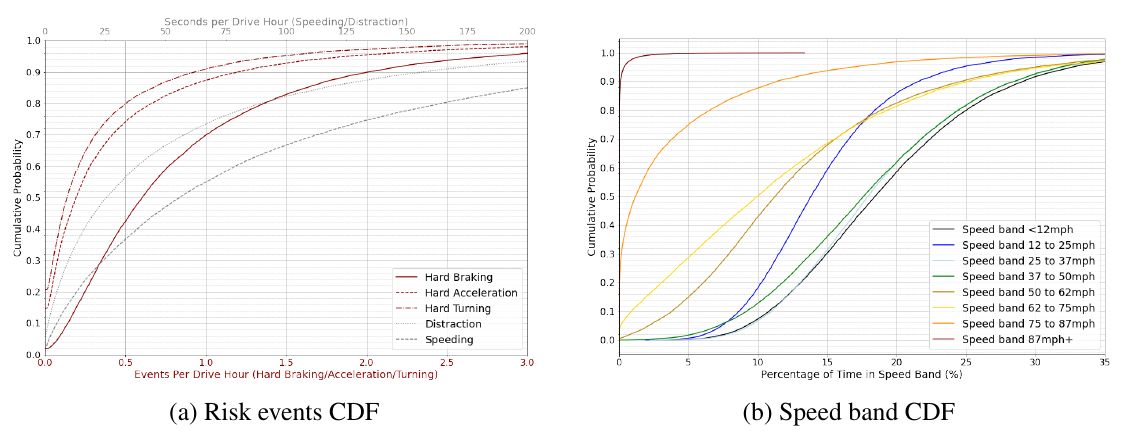
For the 14K drivers analyzed in this study, we plot the prevalence of these risk events in the first month of telematics-measured driving, as shown in the cumulative distribution functions (CDFs) in Fig. 1a. Hard braking is the most frequent risk event per drive hour, more so than hard acceleration and hard turning, and this trend persists across the distribution. Speeding is more common than phone distraction. We also consider time spent in various speed bands, as shown in Fig. 1b. Unlike speeding, which depends on posted limits, time in speed bands can occur regardless of speed limits. Exceeding 85mph is illegal nationwide, with most states having lower limits (40). Most drivers never exceed 87mph, but 25% spend at least 5% of their time driving between 75 and 87mph. The slowest speed band (less than 12mph which includes idling) is the most prevalent, followed by midrange speeds.
We also examine changes in the overall telematics safety behavioral driving score (37). CMT’s Behavioral Score, assessed bi-weekly, provides feedback on individual trips and helps drivers understand their performance. This score, ranging from 40 to 100, integrates the frequency and severity of risk events and is predictive of insurance claims and crashes, summarizing each driver’s safety.
Interpreting Fuel Consumption with Telematics-Measured Driving Behaviors
Next we connect the fuel consumption model outputs with telematics-measured driving behaviors to understand their impact on fuel consumption. The models (CMT-ICE, VT-CPFM, VT-HEV, VT-CPEM) predict fuel usage 15 times per second, necessitating a more interpretable model for quantifying the impacts of driving behavior. We establish a multiple regression using driving behaviors as explanatory variables and the predicted fuel consumption as the response variable. This method links actionable efficiency advice for drivers to the fuel consumption predicted by the detailed models.
Fuel Consumption Regression Specification
We analyze the first month of telematics data for the 14K drivers described earlier. For each driver i and fuel consumption model m, we compute the month one emissions efficiency, Ei,m. Additionally, we quantify driving behaviors, categorizing them into two groups: time spent in specific speed bands (SB) and risky behaviors (hard acceleration, hard braking, hard turning, distraction, and speeding). Time spent in SB j is denoted as Sj, and the prevalence of risk event k is denoted as Rk. These explanatory variables are listed in Table 2. We construct the multiple regression model to relate driving behaviors to emissions efficiency as follows:

Certain speed bands are omitted in Eq. 7 because the total percentage of time spent in all speed bands equals 100%, necessitating the omission of at least one band to prevent multicollinearity. To ensure model robustness, we compute the Variance Inflation Factors (VIF) to check for multicollinearity. A VIF of 1 indicates no correlation, 1-5 suggests moderate correlation, and above 10 indicates significant multicollinearity, affecting coefficient reliability. We ensure all VIF values are below 5 (41). To achieve this, we combined time spent in midrange speed bands, considered the most efficient (11), until the threshold was met.
For each fuel consumption model m, we perform the regression in Eq. 7 in two ways. The first approach allows us to compare the impact of various driving behaviors, and the second maximizes interpretability. To achieve this, we run the regression with and without normalizing the explanatory variables. The first approach uses standard normalization (subtracting the mean and dividing by the standard deviation), resulting in a mean of zero and a standard deviation of one. The second approach uses non-normalized coefficients with units as defined in Table 2. The purpose of including non-normalized coefficients, alongside normalized ones, is to clearly illustrate how changes in driving behavior directly affect emissions. While normalized coefficients can convey this information, they are less intuitive. For example, if the percentage of time spent in a specific speed band were reduced, the efficiency benefit could be calculated from the normalized coefficients, provided the mean and standard deviation of this variable were available to the driver. However, using non-normalized coefficients makes this step unnecessary, as a driver can directly understand how changes in behavior influence emissions.
Safe Driving Behaviors Predictive of Fuel Consumption
Results from the multiple regression, shown in Table 2 and Fig. 2, reveal a strong, significant relationship between the independent variables and predicted fuel consumption. Three models (CMT-ICE, VT-CPFM, VT-HEV) exhibit high R2 values (0.803, 0.830, 0.787). Despite differences in vehicles (SUV vs. sedan), most of the variance in per-driver emissions efficiency is predicted from telematics-measured driving behaviors. The HEV model shows similar results. The BEV model (VT-CPEM) has a moderate R2 value of 0.577. Overall, the regression captures the majority of variability in fuel consumption data across all models.
We first analyze the normalized regression results in Table 2 and Fig. 2 to compare the impact of driving behaviors on emissions efficiency. For all models, driving within specific speed bands is most influential for emissions efficiency, with midrange speeds generally being more efficient (11). Driving below 12mph, including idling, is particularly inefficient for both ICEV and BEV models. For the CMT-ICE and VT-HEV models, driving between 62 and 87mph is also inefficient. However, this inefficiency is not observed in the VT-CPFM and VT-CPEM models.
In all fuel consumption models, hard braking is the most impactful risky behavior for emissions efficiency. This is particularly interesting for the BEV model, where efficiency gains from regenerative braking might be expected. However, the overall effect of sharp deceleration that triggers a hard brake event negates the nuanced efficiency gains from regenerative braking. Except for one minor case, all considered risky behaviors are inefficient, indicated by positive coefficients with 95% confidence intervals. The exception is the distraction coefficient for the VT-CPFM model, which is small but negative, suggesting that increased distraction slightly reduces emissions for this model. The other three models have positive distraction coefficients. This discrepancy is plausible, as distracted drivers may not drive aggressively, thus avoiding fuel waste, but they may still perform abrupt maneuvers due to distraction.
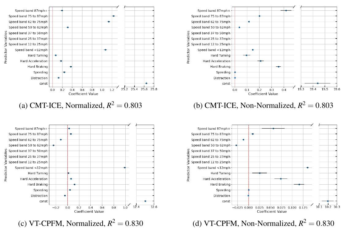
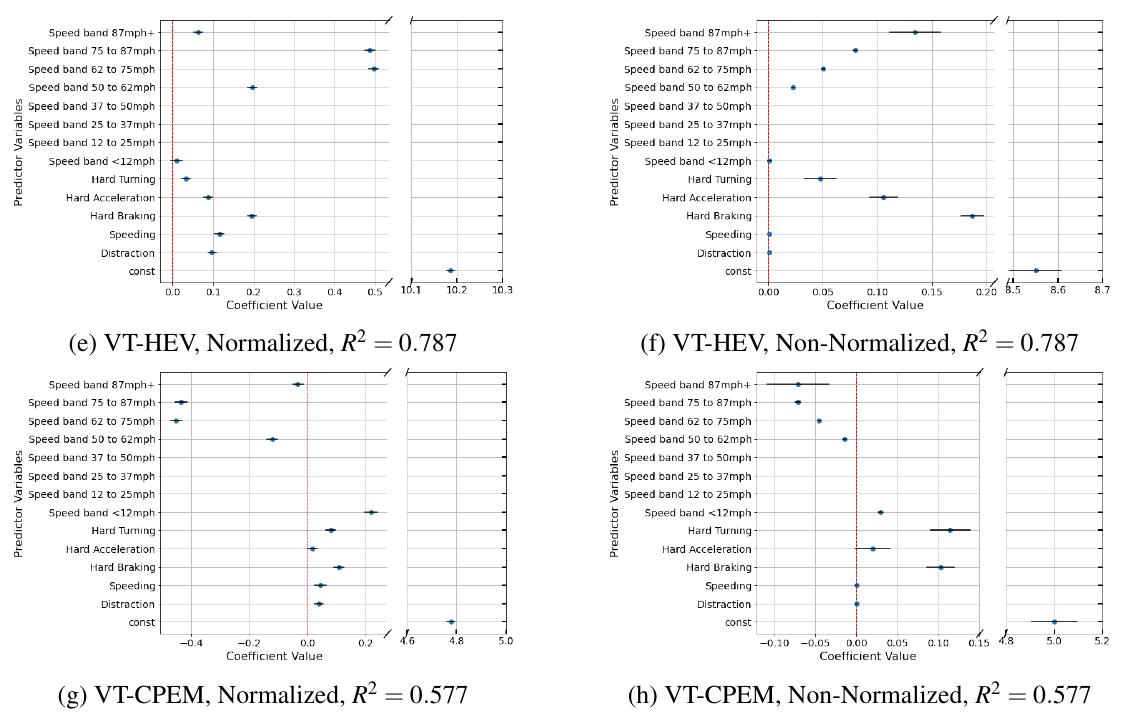
By analyzing the non-normalized regression results in Table 2 and Fig. 2, we gain tangible insights. Increasing hard braking by one event per drive hour results in an average per-driver emission increase of 0.357 kg/100km for the CMT-ICE model (2023 Jeep Grand Cherokee), 0.107 kg/100km for the VT-CPFM model (2024 Toyota Camry), 0.198 kg/100km for the VT-HEV model (2011 Toyota Prius), and 0.114 kg/100km for the VT-CPEM model (2023 Tesla Model Y LR). We can also quantify the impact of reducing time in inefficient speed bands using the non-normalized coefficients. With the 12-50mph band omitted, the results are relative to it. For instance, a driver reducing time in the 75-87mph band from 8% to 2% (a 6% reduction is the standard deviation of this explanatory variable) while increasing time in the 12-50mph band would decrease emissions by 0.202 × 6 = 1.212kg/100km. Assuming an average of 14K miles driven annually, this change saves 273kg GHG per year, or 30.7 gallons of gasoline. This example demonstrates how non-normalized regression results can motivate actionable behavior change.
With the non-normalized explanatory variables, we can directly compare the impact of time spent in various speed bands, as well as time spent distracted versus speeding, and separately the effects of hard acceleration, braking, and turning. However, cross-category comparisons require normalization. Non-normalized results show that driving above 87mph is less efficient than driving at 75-87mph, 62-75mph, or 50-62mph for ICEV or HEV models. This comparison doesn’t hold with normalized variables due to small means and standard deviations for driving above 87mph. Driving below 12mph is inefficient for all models, especially the VT-CPFM model. These findings align with existing literature but present them in a more understandable manner (11).
Finally, we note the unexpected speed band results for the VT-CPEM model. Unlike the other models and existing literature (12), the VT-CPEM regression suggests that driving above 62mph is more efficient than between 12 and 50mph. This surprising finding may be due to the lower R2 value, indicating the model explains less variance in emissions efficiency. Additionally, it’s unclear whether driving above 50mph is inherently less efficient or if there are unaccounted behaviors among drivers at higher speeds. Further investigation with refined models is needed to understand this result.
Impact of Safe Driving Practices on Emissions Efficiency
In this section, we examine how differences in driving performance impact efficiency using the complex fuel consumption models. Building on multiple regression insights from the previous section, we segment the driver population to show that safe driving correlates with fuel efficiency. First, we segment drivers based on their initial month one telematics driving score, which aggregates all risky behaviors. Next, we segment drivers based on changes in their overall telematics driving score from month one to month three, and separately based on changes in hard braking behavior, identified as the most impactful risky behavior for all fuel consumption models. By examining efficiency changes from month one to month three, we gain insights into how emissions efficiency evolves while participating in a telematics program.
To achieve this, we examine the same subset of 14K US drivers. For each driver i, we calculate their month one telematics behavioral score and their month one emissions efficiency (E1i,m), expressed in kg GHG/100km. To analyze how driving behavior correlates with emissions efficiency, we compare the top and bottom deciles of drivers (TD and BD), based on their month one telematics scores. This comparison quantifies the emissions efficiency difference between the initially safest and riskiest drivers. The CDF for these segments, assuming the CMT-ICE model and a 2023 Jeep Grand Cherokee, is shown in Fig. 3.

The distribution separation in Fig. 3 indicates that initially safer drivers are significantly more sustainable than initially riskier drivers. Specifically, the median BD driver emits 26.711 kg GHG/100km, while the median TD driver emits 24.219 kg GHG/100km—a difference of 2.492 kg GHG/100km. This difference translates to 9.9% of the yearly EPA-rated gasoline consumption, or 63.2 gallons of gasoline, assuming the Jeep Grand Cherokee’s EPA rating of 22mpg and 14K annual miles driven. For the 2024 Toyota Camry using the VT-CPFM model, the difference is 0.963 kg GHG/100km, equating to 5.6% (24.4 gallons) of the yearly EPA-rated gasoline consumption. For the 2011 Toyota Prius with the VT-HEV model, the difference is 0.962 kg GHG/100km, equating to 8.4% (24.4 gallons) of the yearly EPA-rated gasoline consumption. For the 2023 Tesla Model Y LR with the VT-CPEM model, the difference is 0.437 kg GHG/100km, equating to 6.5% (253 kWh) of the yearly EPA-rated battery consumption, approximately 8.5 days of electricity for the average U.S. home (1). Thus, for all four distinct vehicles considered, initially safer drivers save over 5% of the annual EPA-estimated fuel compared to initially risky drivers. These results are statistically significant, as confirmed by the Kolmogorov-Smirnov (KS) test at a 0.05 significance level, which evaluates whether the distributions under the null hypothesis (no distinguishable emissions efficiencies) differ statistically from the alternative by comparing CDFs.
Next we consider the same subset of 14K US drivers but focus on changes in safety and efficiency between the first and third months of driving with telematics. We select drivers from the 25th to 75th percentile (7K drivers) based on their month one telematics behavioral score to avoid biases from regression to the mean. For each driver, we calculate their telematics behavioral score and hard braking rates in months 1 and 3. Additionally, for each driver i and each fuel consumption model m, we compute emissions efficiency for month one (E1i,m) and month three (E3i,m), expressed in kg GHG/100km, based on trips in each month. We then examine the per-driver change in efficiency.

In Eq. 8, the change in efficiency (∆Ei,m) is positive for drivers who reduce their emissions (i.e. become more efficient) and negative for those who increase it (i.e. become less efficient).
To analyze the impact of changes in driving behavior on emissions efficiency, we compare the top and bottom deciles of drivers. Unlike the previous segmentation, this comparison is based on changes in behavioral score from month one to month three. Among the 7K drivers in the middle 50 percentiles based on their month one telematics safety behavioral score, we focus on two segments: the 722 drivers who improved their behavioral score the most (top decile, TD) and the 722 drivers who improved the least (bottom decile, BD).
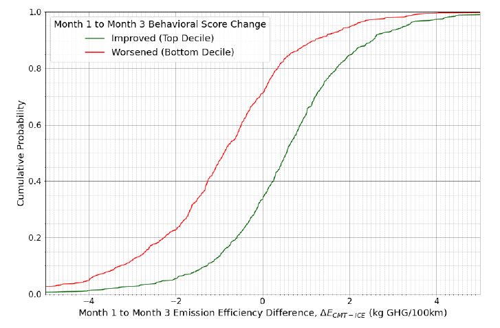
For each fuel consumption model, we calculate the per-driver change in efficiency as defined in Eq. 8 and compare the efficiency change distributions between the TD and BD. The CDF for these segments, assuming the CMT-ICE model and a 2023 Jeep Grand Cherokee, is shown in Fig. 4. The separation in distributions highlights that those who improve their behavioral score also improve their emissions efficiency at higher rates: 66.5% of TD drivers improved, compared to 28.8% of BD drivers. The improvement lift is 2.31, indicating 2.31 times more TD drivers improve than BD drivers. Comparing the distributions shows the median TD driver emits 1.442 kg GHG/100km less than the median BD driver, translating to 36.6 fewer gallons of gasoline annually. This difference represents 5.8% of the yearly EPA-rated gasoline consumption, assuming the Jeep Grand Cherokee’s EPA rating of 22mpg and 14K annual miles driven.
Next, we analyze the 722 drivers who improved their hard braking rate the most (top decile, TD) and the 722 who improved the least (bottom decile, BD) from month one to month three. It is important to note that the TD and BD groups for hard braking segmentation differ from those used for the score change segmentation above. Results for both segmentations across all fuel consumption models are listed in Table 3.
Table 3 shows that drivers who improve in safety also enhance their emissions efficiency. The improvement efficiency lift exceeds one for all models and segmentations, except for the Tesla score segmentation. This exception aligns with the previously observed unexpected speeding result for the VT-CPEM model. The median TD driver becomes more efficient than the median BD driver, with the same VT-CPEM exception. These results are statistically significant, confirmed by the KS test at a 0.05 significance level.
| Jeep Grand Cherokee | Toyota Camry | Toyota Prius | Tesla Model Y LR | |||||
|---|---|---|---|---|---|---|---|---|
| Hard Brake | Score | Hard Brake | Score | Hard Brake | Score | Hard Brake | Score | |
| TD Improved Efficiency (%) | 52.5 | 66.5 | 66.5 | 54.7 | 51.8 | 64.7 | 68.8 | 49.4 |
| BD Improved Efficiency (%) | 33.1 | 28.8 | 32.3 | 46.5 | 35.3 | 28.4 | 37.3 | 55.8 |
| Improvement Lift (TD/BD) | 1.59 | 2.31 | 2.06 | 1.18 | 1.47 | 2.28 | 1.84 | 0.89 |
| TD Medi (∆Em), (kg/100km) | 0.068 | 0.555 | 0.262 | 0.081 | 0.020 | 0.254 | 0.319 | -0.014 |
| BD Medi (∆Em), (kg/100km) | -0.512 | -0.887 | -0.251 | -0.044 | -0.223 | -0.414 | -0.265 | 0.148 |
| Median Difference | 0.579 | 1.442 | 0.514 | 0.125 | 0.244 | 0.668 | 0.584 | -0.162 |
Conclusion
In this study, we quantify the impact of driving behaviors on fuel efficiency using an interpretable model. By applying four distinct fuel consumption models to a large telematics dataset, we develop a multiple regression method to compare and quantify the effects of various driving behaviors on fuel consumption. Our findings show that improvements in safe driving behaviors, such as reduced hard braking and high-speed driving, are strongly associated with reduced fuel consumption across different vehicle models, including ICEVs, HEVs, and BEVs. Using the regression results, we quantify the fuel consumption impact resulting from changes in these unsafe driving behaviors.
By segmenting the driver population, we demonstrate a strong correlation between safe driving and fuel efficiency. This relationship is evident in both initial behavior, as measured by telematics, and in changes in driving performance observed during participation in a telematics program. The difference in initial driving efficiency between the safest and riskiest drivers is substantial, amounting to over 5% of the annual EPA-estimated fuel usage for all four distinct vehicles considered. By examining changes in safety and efficiency during telematics participation for initially midrange-scoring drivers, we show that those who improve their driving performance from a safety perspective save 6% of the annual EPA-estimated gasoline (36.6 gallons) compared to those who regress, assuming the Jeep Grand Cherokee.
These results support implementing UBI programs, which leverage telematics data to provide feedback and financial incentives for safer and more sustainable driving, thereby reducing crash rates and fuel consumption. This study highlights the importance of integrating safety and efficiency measures in driving behavior interventions and policy-making, promoting a comprehensive approach to road safety and environmental sustainability.
References
- U.S. Energy Information Administration, Frequently Asked Questions, 2024.
- Barkenbus, J. N., Eco-driving: An overlooked climate change initiative. Energy policy, Vol. 38, No. 2, 2010, pp. 762–769.
- World Health Organization, Global Status Report on Road Safety 2018. World Health Organization, Geneva, Switzerland, 2018.
- Blincoe, L., P. Ted R. Miller, M. Jing-Shiarn Wang, P. David Swedler, P. Tristan Coughlin, P. Bruce Lawrence, P. Feng Guo, P. Sheila Klauer, and P. Thomas Dingus, The economic and societal impact of motor vehicle crashes, 2019 (Revised) (Report No. DOT HS 813 403). National Highway Traffic Safety Administration, 2023.
- Sivak, M. and B. Schoettle, Eco-driving: Strategic, tactical, and operational decisions of the driver that influence vehicle fuel economy. Transport Policy, Vol. 22, 2012, pp. 96–99.
- Alam, M. S. and A. McNabola, A critical review and assessment of Eco-Driving policy & technology: Benefits & limitations. Transport Policy, Vol. 35, 2014, pp. 42–49.
- Barth, M. and K. Boriboonsomsin, Energy and emissions impacts of a freeway-based dynamic eco-driving system. Transportation Research Part D: Transport and Environment, Vol. 14, No. 6, 2009, pp. 400–410.
- Van Mierlo, J., G. Maggetto, E. Van de Burgwal, and R. Gense, Driving style and traffic measures-influence on vehicle emissions and fuel consumption. Proceedings of the Institution of Mechanical Engineers, Part D: Journal of Automobile Engineering, Vol. 218, No. 1, 2004, pp. 43–50.
- Thomas, J., S. Huff, B. West, and P. Chambon, Fuel consumption sensitivity of conventional and hybrid electric light-duty gasoline vehicles to driving style. SAE International Journal of Fuels and Lubricants, Vol. 10, No. 3, 2017, pp. 672–689.
- El-Shawarby, I., K. Ahn, and H. Rakha, Comparative field evaluation of vehicle cruise speed and acceleration level impacts on hot stabilized emissions. Transportation Research Part D: Transport and Environment, Vol. 10, No. 1, 2005, pp. 13–30.
- Huang, Y., E. C. Ng, J. L. Zhou, N. C. Surawski, E. F. Chan, and G. Hong, Eco-driving technology for sustainable road transport: A review. Renewable and sustainable energy reviews, Vol. 93, 2018, pp. 596–609.
- Sanguinetti, A., K. Kurani, and J. Davies, The many reasons your mileage may vary: Toward a unifying typology of eco-driving behaviors. Transportation Research Part D: Transport and Environment, Vol. 52, 2017, pp. 73–84.
- Ericsson, E., Independent driving pattern factors and their influence on fuel-use and exhaust emission factors. Transportation Research Part D: Transport and Environment, Vol. 6, No. 5, 2001, pp. 325–345.
- Reinhardt, E., EcoDrive in Switzerland: A success story of Energy 2000. In EcoDrive Conference proceedings, Graz, Austria, 1999, pp. 56–61.
- Elvik, R., Rewarding safe and environmentally sustainable driving: systematic review of trials. Transportation Research Record, Vol. 2465, No. 1, 2014, pp. 1–7.
- Young, M. S., S. A. Birrell, and N. A. Stanton, Safe driving in a green world: A review of driver performance benchmarks and technologies to support ‘smart’ driving. Applied ergonomics, Vol. 42, No. 4, 2011, pp. 533–539.
- Dingus, T. A., F. Guo, S. Lee, J. F. Antin, M. Perez, M. Buchanan-King, and J. Hankey, Driver crash risk factors and prevalence evaluation using naturalistic driving data. Proceedings of the National Academy of Sciences, Vol. 113, No. 10, 2016, pp. 2636–2641.
- Arumugam, S. and R. Bhargavi, A survey on driving behavior analysis in usage based insurance using big data. Journal of Big Data, Vol. 6, 2019, pp. 1–21.
- Soleymanian, M., C. B. Weinberg, and T. Zhu, Sensor Data and Behavioral Tracking: Does Usage-Based Auto Insurance Benefit Drivers? Marketing Science, Vol. 38, 2019, pp. 21–43.
- Pinals, L., A. Kerin, C. Van Alsten, R. Sharp, and S. Madden, Motivating Safer Driving with Telematics. In Transportation Research Board Annual Meeting, Washington, D.C., 2024.
- Zhou, M., H. Jin, and W. Wang, A review of vehicle fuel consumption models to evaluate eco-driving and eco-routing. Transportation Research Part D: Transport and Environment, Vol. 49, 2016, pp. 203–218.
- Zheng, J. and Y. Wu, Development of a Practical Method to Estimate the Eco-Level of Driver Performance. Journal of Advanced Transportation, Vol. 2020, No. 1, 2020, p. 8151720.
- Lois, D., Y. Wang, A. Boggio-Marzet, and A. Monzon, Multivariate analysis of fuel consumption related to eco-driving: Interaction of driving patterns and external factors. Transportation Research Part D: Transport and Environment, Vol. 72, 2019, pp. 232–242.
- Wang, Z., M. Mae, S. Nishimura, and R. Matsuhashi, Vehicular Fuel Consumption and CO2 Emission Estimation Model Integrating Novel Driving Behavior Data Using Machine Learning. Energies, Vol. 17, No. 6, 2024, p. 1410.
- United States Environmental Protection Agency, Greenhouse Gas Emissions from a Typical Passenger Vehicle. https://www.epa.gov/greenvehicles/greenhouse-gas-emissions-typical-passenger-vehicle, 2023, accessed: 2024-07-03.
- Gennaro, M. D. et al., Experimental Test Campaign on a Battery Electric Vehicle: Laboratory Test Results (Part 1). SAE International Journal of Alternative Powertrains, Vol. 4, No. 2015-01-1167, 2015, pp. 100–114.
- Department of Energy (DOE), Advanced Vehicle Testing Activity (AVTA) of the Idaho National Laboratory (INL). http://avt.inel.gov/pdf/fsev/fact2013nissanleaf.pdf, 2013, accessed: 2015-06-30.
- Nissan Leaf, Nissan Leaf Characteristics. http://www.nissanusa.com/electric-cars/leaf/, 2015, accessed: 2015-06-30.
- Cambridge Mobile Telematics Launches Driving Scores for Fuel Consumption and CO2 Emissions. https://www.cmtelematics.com/, 2024.
- Hallauer, T., Making Auto Insurance Sustainable. https://www.cmtelematics.com/making-auto-insurance-sustainable-report/, 2023.
- Rakha, H. A., K. Ahn, K. Moran, B. Saerens, and E. V. den Bulck, Virginia tech comprehensive power-based fuel consumption model: model development and testing. Transportation Research Part D: Transport and Environment, Vol. 16, No. 7, 2011, pp. 492–503.
- Ahn, K. and H. A. Rakha, A Simple Hybrid Electric Vehicle Fuel Consumption Model for Transportation Applications. In Electric and Hybrid Vehicles, 2019.
- Fiori, C., K. Ahn, and H. A. Rakha, Power-based electric vehicle energy consumption model: Model development and validation. Applied Energy, Vol. 168, 2016, pp. 257–268.
- SAE International, 2011 Nissan Leaf Vehicle Overview. http://c.ymcdn.com/sites/www.electricauto.org/resource/resmgr/media/nissan_leaf_sae_2_11.pdf, 2011, accessed: 2015-07-14.
- U.S. Department of Energy, Fuel Economy. https://www.fueleconomy.gov, 2024, accessed: 2024-07-03.
- U.S. Department of Transportation, Federal Highway Administration, 2022 National Household Travel Survey Summary of Travel Trends. https://nhts.ornl.gov/assets/2022/pub/2022_NHTS_Summary_Travel_Trends.pdf, 2022, accessed: 2024-07-05.
- Balakrishnan, H., W. Bradley, S. R. Madden, and J. Park, Determining, Scoring, and Reporting Mobile Phone Distraction of a Driver, U.S. Patent US11485369B2, Nov. 2022.
- Malalur, P. G., H. Balakrishnan, and S. R. Madden, Telematics Using Personal Mobile Devices, U.S. Patent US8457880B1, June 2013.
- 2019 Driver Risk Rating Using CMT Data. Tennessee System for Electronic Rate and Form Filing (SERFF), SERFF Tracking Number FRCS-133159732.
- Insurance Institute for Highway Safety (IIHS), Speed Limit Laws, 2024, accessed: 2024-07-15.
- Sheather, S., A modern approach to regression with R. Springer Science & Business Media, 2009.
| CMT-ICE Model | VT-CPFM Model | VT-HEV Model | VT-CPEM Model | |||||
|---|---|---|---|---|---|---|---|---|
| Norm | Non-Norm | Norm | Non-Norm | Norm | Non-Norm | Norm | Non-Norm | |
| Distraction1 R1 | 0.124*** (0.009) | 0.001*** (9.5e-05) | -0.048*** (0.005) | -0.001*** (5.78e-05) | 0.102*** (0.005) | 0.001*** (5.16e-05) | 0.044*** (0.008) | 0.001*** (8.45e-05) |
| Speeding1 R2 | 0.241*** (0.011) | 0.002*** (9.33e-05) | 0.040*** (0.007) | 0.001*** (5.56e-05) | 0.118*** (0.006) | 0.001*** (4.96e-05) | 0.033*** (0.010) | 0.001*** (8.13e-05) |
| Hard Braking2 R3 | 0.372*** (0.010) | 0.357*** (0.010) | 0.112*** (0.006) | 0.107*** (0.006) | 0.206*** (0.006) | 0.198*** (0.005) | 0.119*** (0.009) | 0.114*** (0.009) |
| Hard Accel.2 R4 | 0.175*** (0.010) | 0.211*** (0.012) | 0.066*** (0.006) | 0.079*** (0.008) | 0.089*** (0.006) | 0.107*** (0.007) | 0.017* (0.009) | 0.021* (0.011) |
| Hard Turning2 R5 | 0.068*** (0.010) | 0.097*** (0.014) | 0.026*** (0.006) | 0.037*** (0.008) | 0.028*** (0.005) | 0.040*** (0.0.007) | 0.077*** (0.008) | 0.110*** (0.012) |
| SB <12mph3 S1 | 1.069*** (0.013) | 0.146*** (0.002) | 0.990*** (0.008) | 0.135*** (0.001) | 0.015** (0.007) | 0.002** (0.001) | 0.227*** (0.011) | 0.031*** (0.002) |
| SB 12-25mph3 | ||||||||
| SB 25-37mph3 | ||||||||
| SB 37-50mph3 | ||||||||
| SB 50-62mph3 S2 | 0.309*** (0.011) | 0.0361*** (0.001) | -0.240*** (0.006) | -0.028*** (0.001) | 0.198*** (0.006) | 0.023*** (0.001) | -0.115*** (0.009) | -0.013*** (0.001) |
| SB 62-75mph3 S3 | 1.137*** (0.011) | 0.115*** (0.001) | -0.115*** (0.006) | -0.012*** (0.001) | 0.500*** (0.006) | 0.051*** (0.001) | -0.453*** (0.009) | -0.046*** (0.001) |
| SB 75-87mph3 S4 | 1.232*** (0.011) | 0.202*** (0.002) | 0.060*** (0.007) | 0.010*** (0.001) | 0.483*** (0.006) | 0.080*** (0.001) | -0.431*** (0.010) | -0.071*** (0.002) |
| SB 87mph+3 S5 | 0.195*** (0.010) | 0.419*** (0.022) | 0.026*** (0.006) | 0.057*** (0.012) | 0.060*** (0.005) | 0.130*** (0.011) | -0.032*** (0.008) | -0.070*** (0.017) |
| _cons | 25.643*** (0.009) | 19.438*** (0.054) | 12.507*** (0.005) | 10.201*** (0.032) | 10.185*** (0.005) | 8.523*** (0.029) | 4.779*** (0.007) | 4.965*** (0.047) |
| Obs. | 11545 | 11545 | 11545 | 11545 | 11545 | 11545 | 11545 | 11545 |
| R-squared | 0.803 | 0.803 | 0.830 | 0.830 | 0.787 | 0.787 | 0.577 | 0.577 |
Standard errors are in parentheses. *** p<0.01, ** p<0.05, * p<0.1
1 Non-normalized units are seconds per drive hour.
2 Non-normalized units are events per drive hour.
3 Non-normalized units are percentage of time in speed band (%)
Questions and answers
Answers are quoted from the report.
Does safe driving save fuel?
Our findings show that improvements in safe driving behaviors, such as reduced hard braking and high-speed driving, are strongly associated with reduced fuel consumption across different vehicle models, including ICEVs, HEVs, and BEVs.
How much less fuel do safe drivers use than risky drivers?
Thus, for all four distinct vehicles considered, initially safer drivers save over 5% of the annual EPA-estimated fuel compared to initially risky drivers.
How much gasoline can a driver save by improving their driving score?
Comparing the distributions shows the median TD driver emits 1.442 kg GHG/100km less than the median BD driver, translating to 36.6 fewer gallons of gasoline annually. This difference represents 5.8% of the yearly EPA-rated gasoline consumption, assuming the Jeep Grand Cherokee’s EPA rating of 22mpg and 14K annual miles driven.
Which risky driving behavior wastes the most fuel?
In all fuel consumption models, hard braking is the most impactful risky behavior for emissions efficiency.
Does hard braking hurt efficiency in an electric vehicle?
This is particularly interesting for the BEV model, where efficiency gains from regenerative braking might be expected. However, the overall effect of sharp deceleration that triggers a hard brake event negates the nuanced efficiency gains from regenerative braking.
Which driving speeds use the most fuel?
Non-normalized results show that driving above 87mph is less efficient than driving at 75-87mph, 62-75mph, or 50-62mph for ICEV or HEV models. Driving below 12mph is inefficient for all models, especially the VT-CPFM model.
What is eco-driving?
Eco-driving refers to the decisions a driver makes to improve fuel economy and reduce environmental impact. These include strategic choices, such as vehicle selection and maintenance; tactical choices, like route selection; and operational choices, including driver behavior (5).
How was this measured and which drivers were studied?
We analyze 14,432 randomly selected US-based drivers in various telematics programs, with their first telematics trip between July 1, 2021, and July 1, 2022. We processed 1.5 million trips from both month one and month three for these drivers using the four fuel consumption models, assuming flat terrain.